Week 7 - Modeling Sequences with RNNs

7a - Modeling sequences: A brief overview

7a-02 - Getting targets when modeling sequences

7a-03 - Memoryless models for sequences

7a-04 - Beyond memoryless models

7a-05 - Linear Dynamical Systems (engineers love them!)

• 7a 5:50
• 
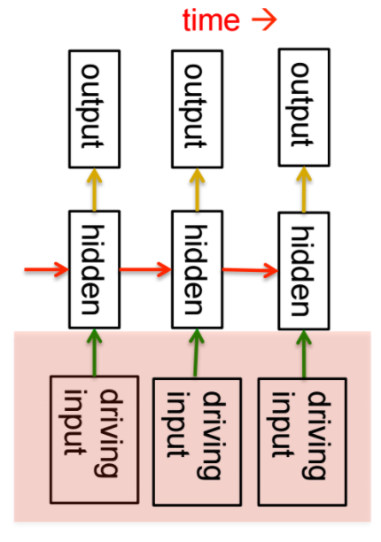
• real-valued hidden state with linear dynamics shown by red arrows above
• the hidden state evolves probabilistically
• there may be driving input influencing hidden state directly (green arrows above)
• we need to be able to infer the hidden states
• used for tracking missiles
• gauss used this for tracking planets assuming a certain type of noise (Gaussian noise)
• distribution over hidden state given data is Gaussian
  • can be computed using "Kalman filtering"
• given observations of the output of the system, we can't know for sure what was happening inside, but we can infer with a certain probability what was going on

7a-06 - Hidden Markov Models (computer scientists love them!)

• 7a 8:19
• 
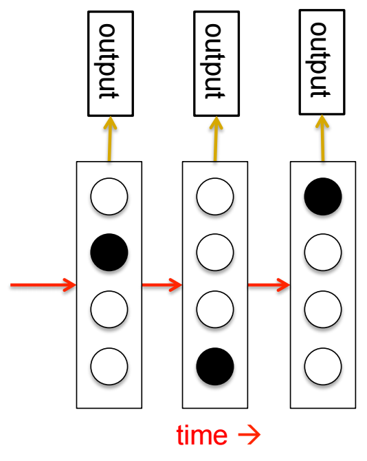
• The hidden state consists of a one-of-N choice.
• System is always in exactly one of those states.
• Transitions controlled by transition matrix: a matrix of probabilities.
• The output model is stochastic. The state that the system is in doesn't completely determine what output it produces. There is some variation in the output that each output can produce.
• We can't be sure which state produced which output - the states are hidden "behind a veil"
• It is easy to represent a probability distribution across N states with N numbers
• Even though we can't know what state it's in for sure, we can easily represent the probability distribution.
• To predict the next output from the HMM, we need to predict what hidden state it is probably in, and so we need to get our hands on that probability distribution.
• There is a method based on Dynamic Programming that lets us take observations we've made and from those compute the probabitity dist across hidden states
• Once we have the probability dist, there's a learning algorithm for HMMs and that's what make them appropriate for speech. In 1970 they took over speech recognition.

7a-06 - Hidden Markov Models notes and comments

• I believe that Hinton means that a HMM network has one unit for each state for each timestamp. He doesn't really say that, though.
• This part is a little confusing, because technically, if you have N states that are numbered 1 through N, you could have a single unit per time slot that selected the integer for each time slot

7a-07 - A fundamental limitation of HMMs

• 7a 10:32
• It's easiest to understand the limitations of HMM if we consider what happens when an HMM generates data.
• At each time step it selects one of its discrete hidden states.
• Consider that each of its N hidden states could be referred to by a single integer. That integer can be represented in log N bits.
• At each time stamp, that slice of the HMM only knows which integer was selected by the immediately prior time stamp.
• Therefore each time slice of an HMM system with N states only has access to log N bits of memory about what has transpired before it.

7a-08 - Recurrent neural networks

• 12:56
• They have distributed state
  • several units can be active at once so they can remember several different things at once
  • "They are nonlinear"
  • "a linear dynamical system has a whole hidden state vector"
  • "it's got more than one value at a time,"
  • "but those values are constrained to act in a linear way so as to make inference easy,"
  • "and in a recurrent neural network we allow the dynamics to be much more complicated."
  • "non-linear dynamics" allows them "to update their hidden state in complicated ways" (?)
• with enough neurons and enough time, a RNN can mimic any computer

7a-08 - RNNs Notes and Comments

• It's unclear to me whether he's talking about RNNs, HMMs, LDSs, all three, or just one. The slide title is Recurrent Neural Networks, but it seems as though he is saying things only about Linear Dynamical Systems, because
• HMMs don't have more than one state active at once
• But how do linear dynamical systems exhibit "non-linear dynamics"?

7a-09 - Do generative models need to be stochastic?

• compare the distribution of an HMM to the hidden state of an LDS

7a-10 - Recurrent neural networks

• behavior they can exhibit
  • can oscillate
  • can settle to point attractors (retrieving memories?)
    • hopfield networks
  • behave chaotically (bad for information processing?)
  • can potentially learn to implement lots of small programs that run in parallel and interact in complicated ways
• drawbacks
  • computational power of RNNs makes them very hard to train
    • one successful example: Tony Robinson's speech recognizer which uses "transputers"

7b - Training RNNs with backpropagation

7b-02 - The equivalence between feedforward nets and recurrent nets

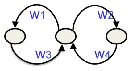
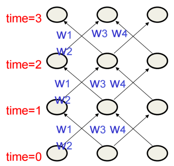
• assume that there is a time delay of 1 in using each connection
• the recurrent net is just a layered net that keeps reusing the same weights.

7b-03 - Reminder: Backpropagation with weight constraints

• it is easy to modify backprop to incorporate constraints between weights
• compute gradients as usual then modify them so they satisfy constraints
• if they started off satisfying them, they will continue to satisfy them
• to constrain $w_{1,\text{t=0}} = w_{1,\text{t=1}}$
• we need: $\Delta w_{1,\text{t=0}} = \Delta w_{1,\text{t=1}}$
• compute: $\frac{\partial E}{\partial w_{1,\text{t=0}}} \text{and} \frac{ \partial E }{ \partial w_{1,\text{t=1}} }$
• then, use $\frac{\partial E}{\partial w_{1,\text{t=0}}} + \frac{ \partial E }{ \partial w_{1,\text{t=1}} }$ for both $w_{1,\text{t=0}}$ and $w_{1,\text{t=1}}$.

7b-04 - Backpropagation through time

Training algorithm in the time domain:

– The forward pass builds up a stack of the activities of all the units at each time step. – The backward pass peels activities off the stack to compute the error derivatives at each time step. – After the backward pass we add together the derivatives at all the different times for each weight.

7b-05 - An irritating extra issue

7b-06 - Providing input to recurrent networks

7b-07 - Teaching signals for recurrent networks

7c - A toy example of training an RNN

7c-02 - A good toy problem for a recurrent network

7c-03 - The algorithm for binary addition

7c-04 - A recurrent net for binary addition

7c-05 - The connectivity of the network

7c-06 - What the network learns

• RNNs can emulate finite state automaton, but they are more powerful than FSAs
  • with N hidden neurons, it has $2^N$ binary activity vectors
  • it still has only $N^2$ weights
  • when the imput stream has two things going on at once, this "is important"
  • A finite state automaton "needs to square its number of states"
  • An RNN "needs to double it's number of units"

7d - Why it is difficult to train an RNN

7d-02 - The backward pass is linear

7d-03 - The problem of exploding or vanishing gradients

7d-04 - Why the back-propagated gradient blows up

7d-05 - Four effective ways to learn an RNN

7e - Long term short term memory

7e-02 - Long Short Term Memory (LSTM)

7e-03 - Implementing a memory cell in a neural network

7e-04 - Backpropagation through a memory cell

• At initial time, let's assume that keep gate is 0 and write gate is 1
• value of 1.7 from rest of NN is set to 1.7.

7e-05 - Reading cursive handwriting

• natural task for RNN
• usually, input is sequence of (x, y, p) coordinates of the tip of the pen, where p indicates pen up or pen down
• output is sequence of characters.

7e-06 - A demonstration of online handwriting recognition by an RNN with Long Short Term Memory

• from Alex Graves
• movie demo:
• Row 1: This shows when the characters are recognized. – It never revises its output so difficult decisions are more delayed.
• Row 2: This shows the states of a subset of the memory cells. – Notice how they get reset when it recognizes a character.
• Row 3: This shows the writing. The net sees the x and y coordinates. – Optical input actually works a bit better than pen coordinates.
• Row 4: This shows the gradient backpropagated all the way to the x and
  • y inputs from the currently most active character. – This lets you see which bits of the data are influencing the decision.

Week 7 Quiz

Week 7 Quiz - Q1

1. How many bits of information can be modeled by the vector of hidden activities (at a specic time) of a Recurrent Neural Network (RNN) with 16 logistic hidden units?
   1. 2
   2. 4
   3. 16
   4. >16
2. How many bits of information can be modeled by the hidden state (at some specific time) of a Hidden Markov Model with 16 hidden units?
   1. 2
   2. 4
   3. 16
   4. >16

Q1 Notes

• 7c-06 - What the network learns
  • "an RNN with n hidden neurons has $2^{n}$ possible binary activity vectors (but only $n^{2}$ weights)"
  • "A finite state automaton needs to square its number of states" while "An RNN needs to double its number of units."
• With Q1-1, the vector of hidden activities "has $2^n$ possible binary activity vectors" which is much greater than 16.
• With Q1-2, an HMM represents its states with integers. For example, if there are 16 possible states, it takes 4 bits to represent those 16 states, since $2^4$ is 16.
  • Does this imply that HMMs usually have the same number of hidden states as the number of hidden units? There is unexplained context to this question that I'm not picking up.
  • Reading back through 7a-06 - Hidden Markov Models and the following slide, I think that Hinton is implying that if there are 16 states, then there are 16 hidden units per time slot and only one of them is active at a time, either that, or there is one hidden unit per time slot and it outputs an integer from 1 to 16.
  • The important part is that the memory is constrained to log N bits for N states with an HMM.
  • Forum: Difference between HMM and RNN

    • The state vector of an HMM is generated from a multinomial probability distribution over N state values--that's why it can only carry log2N bits of information. The state vector of an RNN with logistic hidden activations is generated from N probability distributions over binary state values.

    • RNNs can have dedicated outputs leaving the hidden states a black box whereas in HMMs the states are usually assigned interpretations ahead of time. In an HMM you can incorporate long-term dependencies by explicitly representing them in the the states and transitions leading to very large and sparse transition matrices--very typical in speech and language processing. Leaving the hidden states a black box allows the model to learn to encode long-term information on its own.

Week 7 Quiz - Q2

This question is about speech recognition. To accurately recognize what phoneme is being spoken at a particular time, one needs to know the sound data from 100ms before that time to 100ms after that time, i.e. a total of 200ms of sound data. Which of the following setups have access to enough sound data to recognize what phoneme was being spoken 100ms into the past?

1. A feed forward Neural Network with 200ms of input
2. A Recurrent Neural Network (RNN) with 200ms of input
3. A feed forward Neural Network with 30ms of input
4. A Recurrent Neural Network (RNN) with 30ms of input

Q2 Notes

• it's only recurrent neural networks that can reasonably simulate a finite state automaton by storing information

Week 7 Quiz - Q3

The figure below shows a Recurrent Neural Network (RNN) with one input unit x, one logistic hidden unit $h$, and one linear output unit $y$. The RNN is unrolled in time for T=0, 1, and 2.

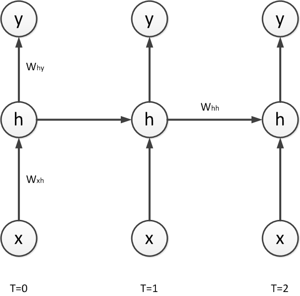
The network parameters are: $W_{xh}=0.5$, $W_{hh}=-1.0$, $W_{hy}=-0.7$, $h_{bias}=-1.0$, and $y_{bias}=0.0$. Remember, $\sigma(k) = \frac{1}{1+\exp(-k)}$.

If the input $x$ takes the values 9, 4, -2 at the time steps 0, 1, 2 respectively, what is the value of the hidden state $h$ at $T=2$? Give your naswer with at least two digits after the decimal point.

Week 7 Quiz - Q3 Work

Week 7 Quiz - Q4

The figure below shows a Recurrent Neural Network (RNN) with one input unit x, one logistic hidden unit h, and one linear output unit. The RNN is unrolled in time for T=0, 1, and 2.

The network parameters are: $W_{xh} =−0.1$, $W_{hh}=0.5$, $W_{hy}=0.25$, $h_{bias}=0.4$, and $y_{bias}=0.0$.

If the input x takes the values 18, 9, −8 at time steps 0, 1, 2 respectively, the hidden unit values will be 0.2, 0.4, 0.8 and the output unit values will be 0.05, 0.1, 0.2 (you can check these values as an exercise).

A variable z is defined as the total input to the hidden unit before the logistic nonlinearity.

If we are using squared error loss with targets t0 = 0.1, t1 = -0.1, t2 = -0.2, what is the value of the error derivative just before the hidden unit nonlinearity at T=2 (i.e. $\frac{\delta E}{\delta z_2}$)? Write your answer up to at least the fourth decimal place.

Week 7 Quiz - Q4 Work

I've adapted prob3.m to prob4's parameters:

Plan: backpropagate to find $\frac{ \partial E }{ \partial z_1 }$.

$$\frac{ \partial E }{ \partial z_1 } = \frac{ \partial E_1 }{ \partial z_1 } + \frac{ \partial E_2 }{ \partial z_1 }$$

Expanding E1 w.r.t. z1: $$\frac{ \partial E_1 }{ \partial z_1 } = \frac{ \partial E }{ y_1 } \frac{ \partial y_1 }{ \partial h_1 } \frac{ \partial h_1 }{ \partial z_1 }$$

Expanding E2 w.r.t. z1 $$\frac{ \partial E_2 }{ \partial z_1 } = \frac{ \partial E_2 }{ \partial y_2 } \frac{ \partial y_2 }{ \partial h_2 } \frac{ \partial h_2 }{ \partial z_2 } \frac{ \partial z_2 }{ \partial h_1 } \frac{ \partial h_1 }{ \partial z_1 }$$

E1 w.r.t. z1

We are using squared error, which means that for each output unit, the error is computed as one half the square of the residual, which is the difference between the target output and the actual output for the unit:

$E_{ j \in \text{all output units} } = \frac{ 1 }{ 2 }(t_j - y_j)^{2}$

So by the chain rule and the power rule,

$$\frac{ \partial E_j }{ \partial y_j } = y_j - t_j$$

$$\frac{ \partial E_1 }{ \partial z_1 } = (y_1 - t_1) \frac{ \partial y_1 }{ \partial h_1 } \frac{ \partial h_1 }{ \partial z_1 }$$

Next, $\frac{ \partial y_1 }{ \partial h_1 } = W_{hy}$; the derivative of y1 w.r.t. the hidden unit 1 activation is just the weight connecting h1 to y1:

$$\frac{ \partial E_1 }{ \partial z_1 } = (y_1 - t_1) * W_{hy} * \frac{ \partial h_1 }{ \partial z_1 }$$

Finally, $\frac{ \partial h_1 }{ \partial z_1 }$ is the logistic function derivative w.r.t. the logit, $h_1(1 - h_1)$. For a review of this, see week 3's slide, "The derivatives of a logistic neuron."

$$\frac{ \partial E_1 }{ \partial z_1 } = (y_1 - t_1) * W_{hy} * h_1(1 - h_1)$$

Given that $y_1 = 0.1$, $t_1 = -0.1$, $W_{hy} = 0.25$, $h_1 = 0.4$: $$\frac{ \partial E_1 }{ \partial z_1 } = (0.1 - -0.1) * 0.25 * 0.4(1 - 0.4)$$

$$\frac{ \partial E_1 }{ \partial z_1 } = 0.012026$$

E2 w.r.t. z1

$$\frac{ \partial E_2 }{ \partial z_1 } = \frac{ \partial E_2 }{ \partial y_2 } \frac{ \partial y_2 }{ \partial h_2 } \frac{ \partial h_2 }{ \partial z_2 } \frac{ \partial z_2 }{ \partial h_1 } \frac{ \partial h_1 }{ \partial z_1 }$$

$$\frac{ \partial E_2 }{ \partial z_1 } = (y_2 - t_2) * W_{hy} * h_2*(1 - h_2) * W_{hh} * h_1*(1 - h_1)$$

Given that $y_2 = -0.2$, $t_2 = -0.2$, $W_{hy} = 0.25$, $h_2 = 0.8$, $W_{hh} = 0.5$, $h_1 = 0.4$:

$$\frac{ \partial E_2 }{ \partial z_1 } = (0.2 - -0.2) * 0.25 * 0.8*(1 - 0.8) * 0.5 * 0.4 * (1 - 0.4)$$

$$\frac{ \partial E_2 }{ \partial z_1 } = 0.0019$$

So completing,

$$\frac{ \partial E }{ \partial z1 } = \frac{ \partial E_1 }{ \partial z_1 } + \frac{ \partial E_2 }{ \partial z_1 }$$

$$\frac{ \partial E }{ \partial z1 } = 0.012026 + 0.0019080 = 0.013934$$

Week 7 Quiz - Q5

Consider a Recurrent Neural Network with one input unit, one logistic hidden unit, and one linear output unit. This RNN is for modeling sequences of length 4 only, and the output unit exists only at the last time step, i.e. T=3. This diagram shows the RNN unrolled in time:

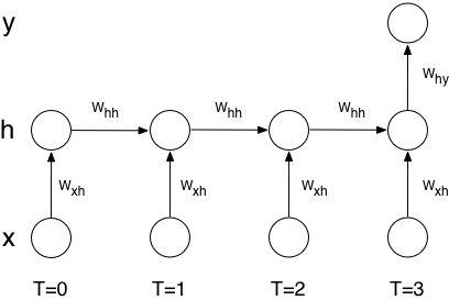
Suppose that the model has learned the following parameter values:

• $w_{xh} = 1$
• $w_{hh} = 2$
• $w_{hy} = 1$
• All biases are 0

For one specific training case, the input is 1 at T=0 and 0 at T=1, T=2, and T=3. The target output (at T=3) is 0.5, and we're using the squared error loss function.

We're interested in the gradient for $w_{xh}$, i.e. $\frac{\partial E}{\partial w_{xh}}$. Because it's only at T=0 that the input is not zero, and it's only at T=3 that there's an output, the error needs to be backpropagated from T=3 to T=0, and that's the kind of situation where RNN's often get either vanishing gradients or exploding gradients. Which of those two occurs in this situation?

You can either do the calculations, and find the answer that way, or you can find the answer with more thinking and less math, by thinking about the slope $\frac{\partial y}{\partial z}$ of the logistic function, and what role that plays in the backpropagation process.

• [A] Vanishing gradient
• [B] Exploding gradient

Week 7 Quiz - Q5 Work

I believe that it will vanish, but I'm not certain why. I'll need to come back and work through the explanation for this one.

Week 7 Vocab

• Attenuation:
• Attractors:
• Unrolled RNN:

Week 7 FAQ

TBD

Week 7 Other

Papers

TBD

Week 7 Links

• PDP Handbook Backpropagation Guide
• Wikipedia: Proportionality ($a \propto b$)
• Swarthmore CS: Derivation of Backpropagation
• Stanford CS Machine Learning: Lecture 1
  • defines squared loss: $_{ \text{Loss}_{\text{squared}} (x, y, w ) } = (f_w(x) - y)^{2}$
• Stanford CS221 Artificial Intelligence: Principles and Techniques
• CS CMU backprop pdf

Week 7 People

Sepp Hochreiter

• researchgate link
• "Long Short-term Memory." Neural Computation 9(8): 1735-80. December 1997. DOI: 10.1162/neco.1997.9.8.1735

Jürgen Schmidhuber

• researchgate link
• "Long Short-term Memory." Neural Computation 9(8): 1735-80. December 1997. DOI: 10.1162/neco.1997.9.8.1735

Alex Graves

• Graves & Schmidhuber (2009) showed that RNNs with LSTM are currently the best systems for reading cursive writing.

Tony Robinson

• Google Scholar Page
• Founder and CEO, Speechmatics